Axonometric Projection#
This section delves into the graphical construction of axonometric images, providing a foundation for understanding the implementation details of the axonometry library.
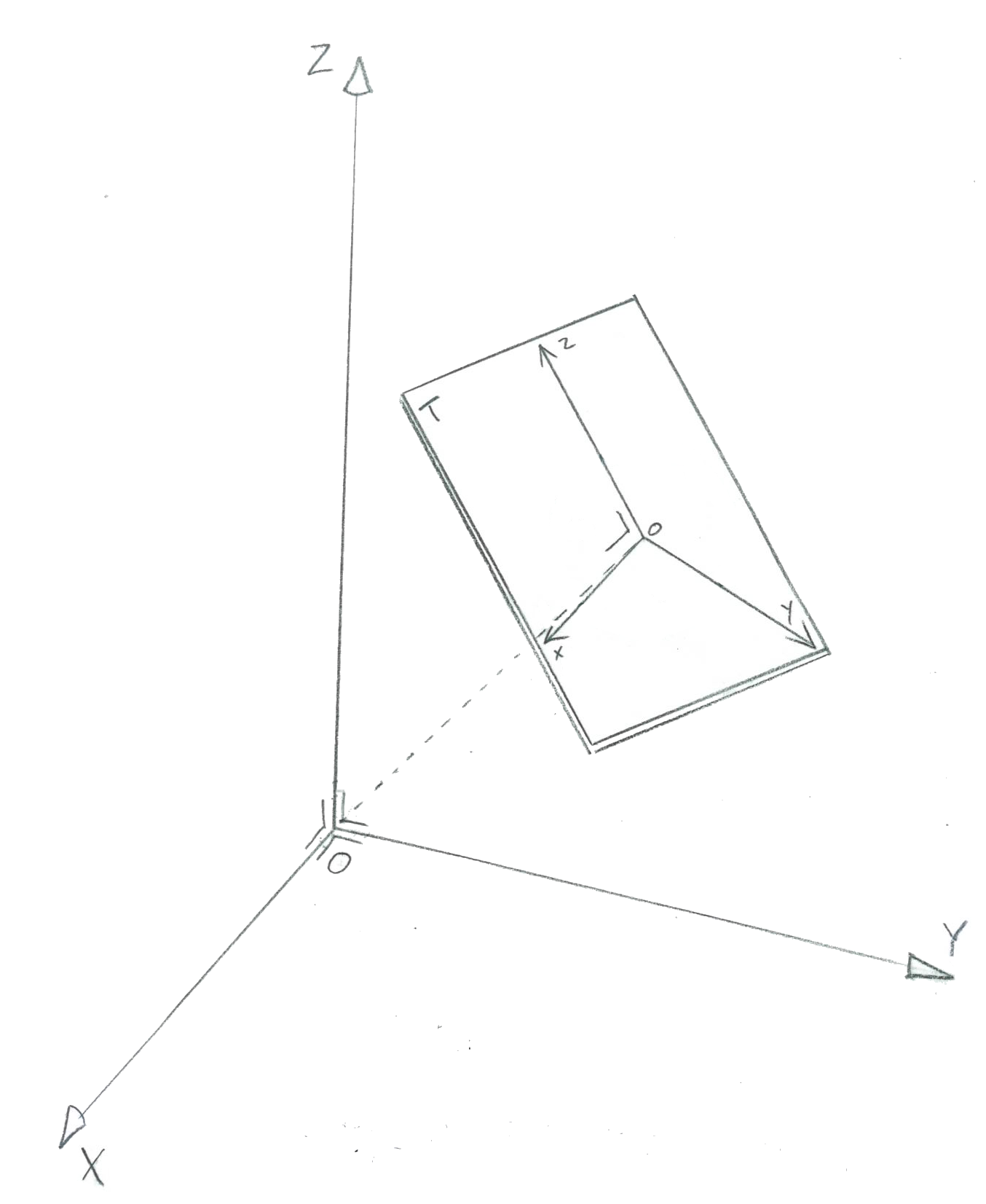
Axonometry is a type of orthogonal projection method, characterized by parallel projection. It involves projecting parallel lines from an object in 3D space onto a separate, parallel projection plane also in space. The key characteristic of axonometry is that the projection lines and the projection plane are always perpendicular (at a strict 90° angle) to each other.
Axonometry allows for the representation of objects in space while preserving certain inherent properties. When an object is projected using axonometry, its length scales remain unchanged, but its angles become distorted. This distortion enables the creation of simplified and more understandable 2D representations of 3D structures.
Orthographic Projection#
A plane in space and projection rays.
Architectural Notation
Note
We use a right-handed coordinate system because it is more common in computer graphics. In architectural drawings, if coordinates are given, a left-handed coordinate system is more common.
Scales#
Unit cube
Nomenclature#
Isometric, Dimetric and Trimetric plus special cases and conventions.
Intersection#
One method to construct an axonometric image is by intersection. It relies on a drawdown operation - a kind of geometric algorithm. It decomposes the axonometric space into three orthogonal planes. The planes are orthogonal views but are in a disposition which enables a geometric relationship with the axonometric image.
To make a drawdown, one relies on the Reference Trihedron, defining the x, y, z space axis. The results are 3 Coordinate Planes (XY, YZ, ZX).
Coordinate Plane Tilt#
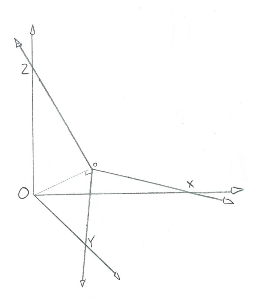
Graphic algorithm to tilt the coordinate planes into the axonometric picture plane.
Reference Plane Disposition Equation#
Solving a Orthodiagonal quadrilateral –> Projection distance = 1
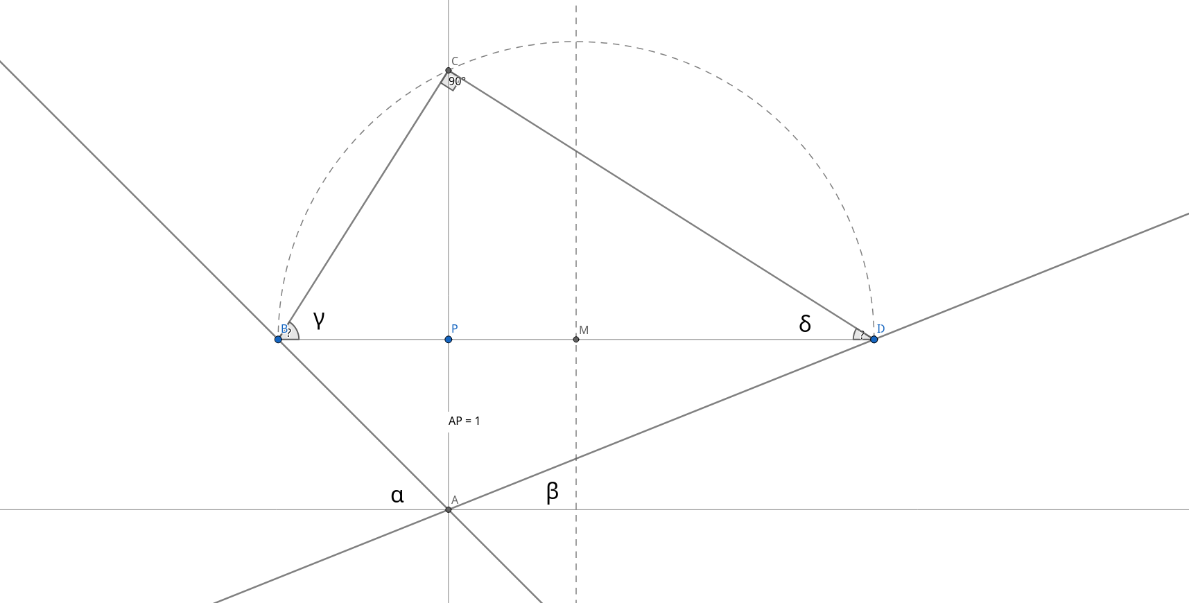
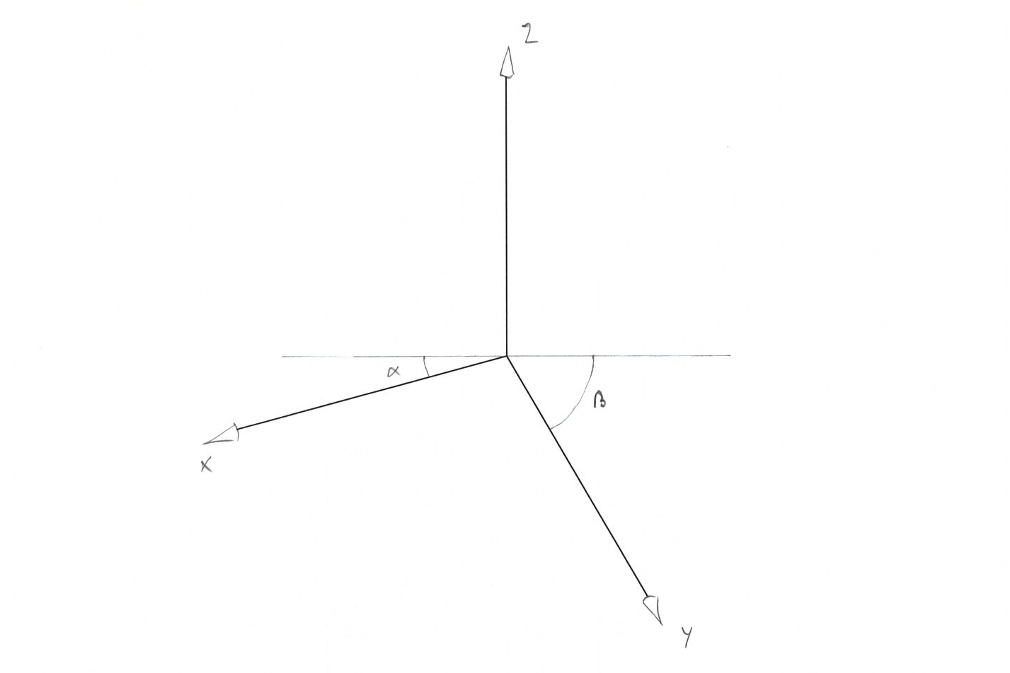
Given \(\alpha\) & \(\beta\) find \(\gamma\) & \(\delta\):
\(\angle XoY = 90{^\circ}\)
\(OP = 1\)
\(XP = \frac{OP}{\tan(\alpha)} = \cot(\alpha)\)
\(YP = \frac{OP}{\tan(\beta)} = \cot(\beta)\)
\(h = \sqrt{XP \ast YP} = \sqrt{\cot(\alpha) \ast \cot(\beta)}\)
\(\gamma = \arctan(\frac{XP}{h}) = \arctan(\frac{\cot(\alpha)}{\sqrt{\cot(\alpha) \ast \cot(\beta)}})\)
\(\delta = \arctan(\frac{YP}{h}) = \arctan(\frac{\cot(\beta)}{\sqrt{\cot(\alpha) \ast \cot(\beta)}})\)