Usage#
This section describes how to use axonometry. Basic Python programming skills are required to use axonometry. Here is a good place to start learning Python.
Hint
The most convenient way to use axonometry is by writing scripts — i.e. text files with a .py extension in which axonometry is imported and then used with a series of commands. To run these scripts use the uv run my_script.py command.
To begin using axonometry in your scripts, add a single line at the top of each file:
from axonometry import *
This imports all public axonometry classes and functions. For a detailed description of everything available in axonometry, please refer to the API Reference section.
Note
When reviewing subsequent listings, note that redundant code parts have been omitted for each listing to focus on key concepts rather than being entire working scripts.
Axonometry Parameters#
The axonometric system is set up when instantiating an Axonometry object with two angles as parameters.
>>> my_axo = Axonometry(41.5, 7)
INFO:axonometry.axonometry:[AXONOMETRY] 41.5°/7°
Hint
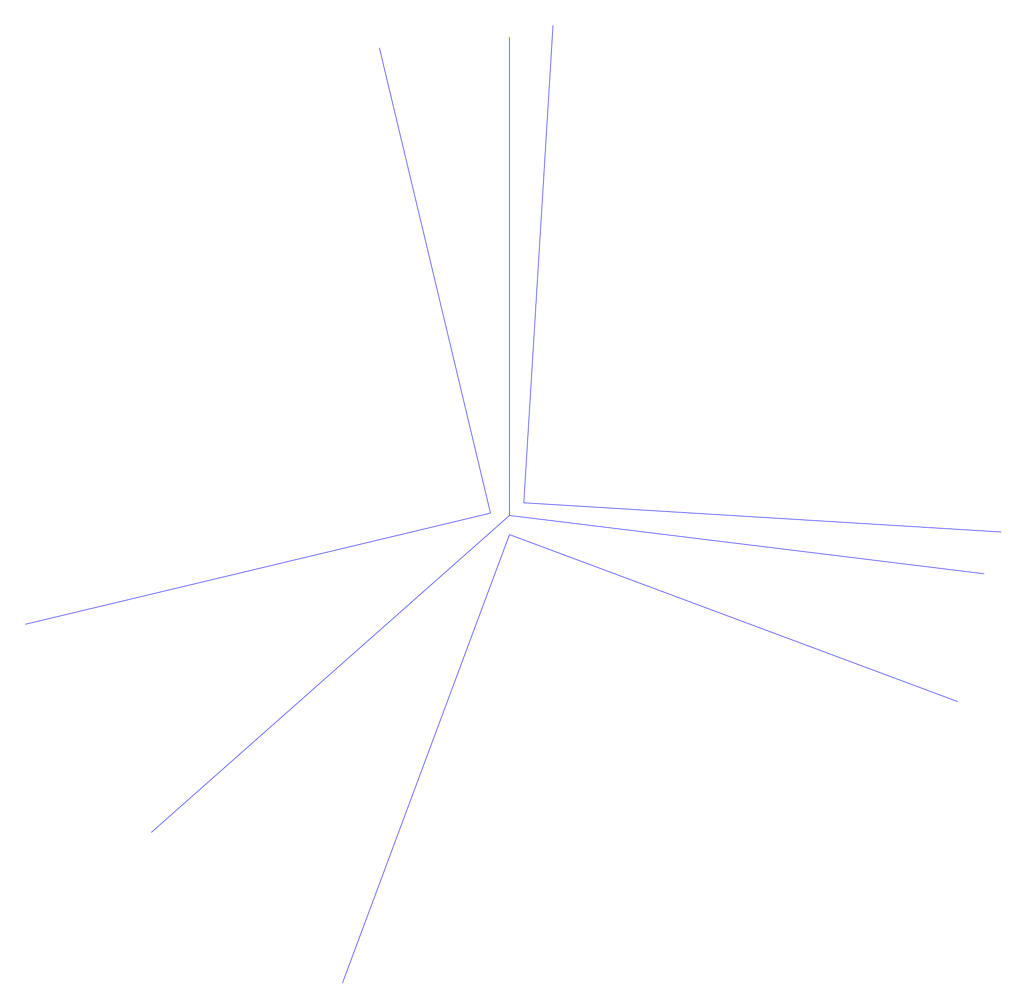
To display the drawing, call the Axonometry.show_paths() method on the my_axo object:
my_axo.show_paths()
Various aspects of the axonometric system can be defined when initializing the Axonometry object and explicitly defining the available parameters. In the listing bellow are shown the default values when initializing an Axonometry object. It does produce exactly the same configuration as the previous listing.
my_axo = Axonometry(41.5,
                    7,
                    ref_planes_distance = 100.0,
                    trihedron_size = 100.0,
                    trihedron_position = (0, 0),
                    page_size = "A1",
                    orientation = "portrait",
                    )
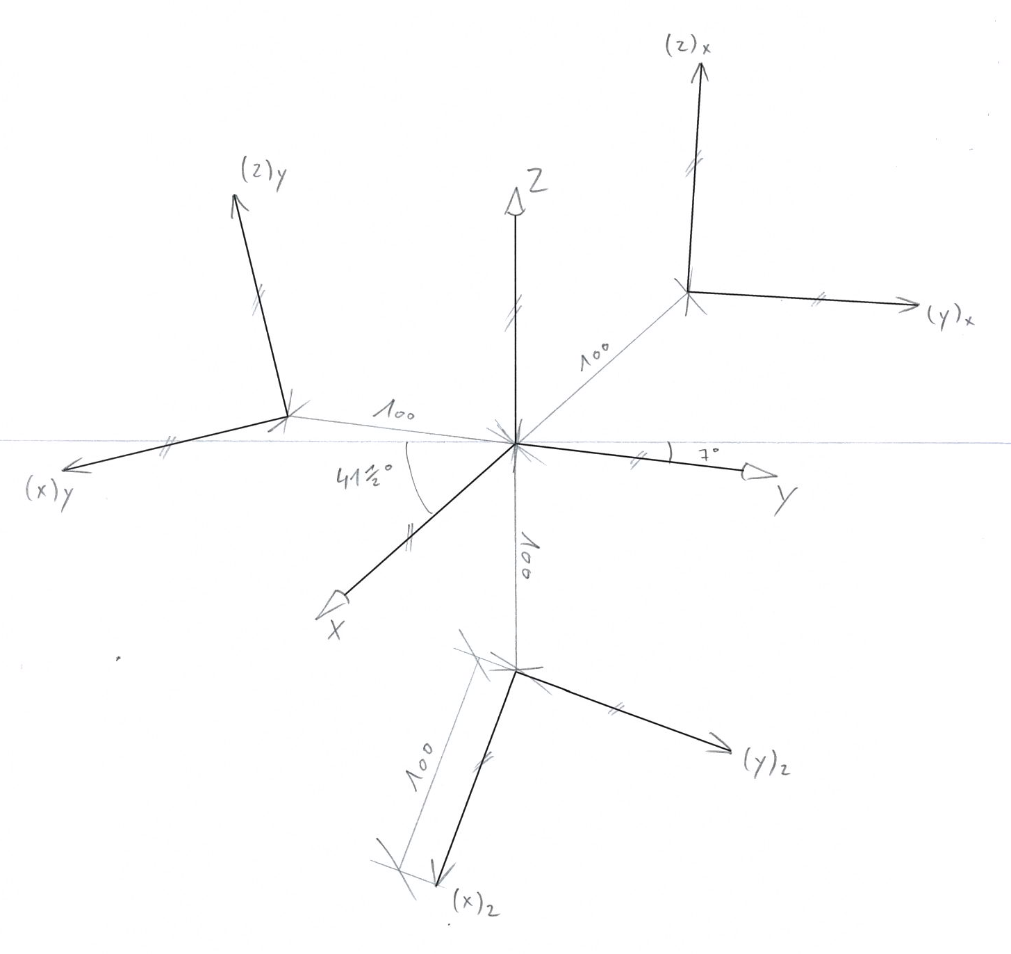
The values mostly defining the projection system are ref_planes_distance and trihedron_size.
Note
The values trihedron_position, page_size and orientation are about where this system is centered on the page and what size that page has. For now, only the default A1 portrait page_size and orientation are implemented. These correspond to our in-house plotter but other as well as the possibility to use custom sizes will be implemented in the future.
The same angle pair but with a ref_planes_distance of 10 and trihedron_size of 250 produces the following configuration.
>>> my_axo = Axonometry(41.5, 7, ref_planes_distance = 10, trihedron_size = 250)
INFO:axonometry.axonometry:[AXONOMETRY] 41.5°/7°
Hint
The Axonometry.random_angles() method accepts exactly the same parameters — minus the angle values.
Resulting Planes#
The drawing functions are tied to the different projection planes. These planes are set up when initializing an Axonometry object. This initializes first makes a Drawing and a Trihedron object, then produces the four Plane objects which are going to be used to start drawing: 1 × Axonometry and 3 × ReferencePlane.
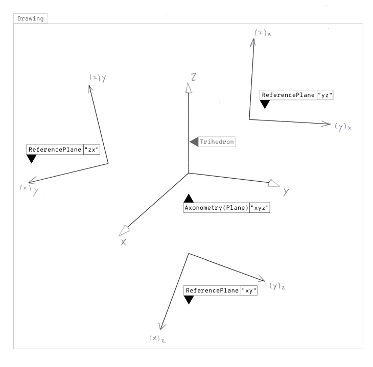
The starting point to begin drawing are these planes: one axonometric picture plane and the three related reference planes. From these planes one can access two methods in order to draw points or lines: Axonometry.draw_point(), Axonometry.draw_line(), ReferencePlane.draw_point(), ReferencePlane.draw_line().
c.f. Implementation
The operation to obtain the three reference planes is called a tilt. The algebraic definition of the tilt and its implementation is a crucial element of the axonometry library.
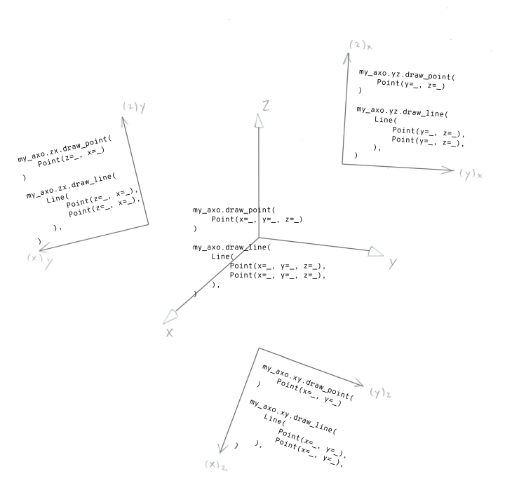
Drawing Methods#
In order to start drawing, it is necessary to access the plane in which you wish to draw. The following diagram illustrates how to access the drawing functions of the different planes, following the same structure as the previous listing.
>>> my_axo = Axonometry(41.5, 7)
INFO:axonometry.axonometry:[AXONOMETRY] 41.5°/7°
my_axo.                           # Axonometry
      ├── draw_point(
      ├── draw_line(
      ├── xy.                     # ReferencePlane
      │     ├── draw_point(
      │     └── draw_line(
      ├── yz.                     # ReferencePlane
      │     ├── draw_point(
      │     └── draw_line(
      └── zx.                     # ReferencePlane
            ├── draw_point(
            └── draw_line(
Another way to illustrate: drawing points and lines in a certain plane is like executing some code in that planes:
Tip
The reference plane objects can also be accessed with a key.
>>> my_axo["xy"]
Reference Plane XY
>>> my_axo["yz"]
Reference Plane YZ
>>> my_axo["zx"]
Reference Plane ZX
Defining Point Objects#
The primary geometric primitive — in regard to plotting — is the Line. To draw lines one defines their start and end with the help of Point objects. Points are initialized in various ways.
Hint
Normally Point and Line has been imported when calling from axonometry import *. Otherwise, both objects can be imported explicitly with from axonometry import Point, Line
With Coordinate Values#
As seen in the previous image, the points’ parameters need to be sepecified explicitly as they correspond to the planes’ coordinate system in which they are drawn.
>>> Point(x=21, y=39, z=56)
Point(x=21.00, y=39.00, z=56.00)
>>> Point(x=29, y=18)
Point(x=29.00, y=18.00)
>>> Point(y=8, z=51)
Point(y=8.00, z=51.00)
>>> Point(z=37, x=49)
Point(x=49.00, z=37.00)
Similarly, points can be made with helper methods for which the argument names can be omitted: Point.from_xyz(), Point.from_xy(), Point.from_yz(), Point.from_zx().
>>> Point.from_xyz(21, 39, 56)
Point(x=21.00, y=39.00, z=56.00)
>>> Point.from_xy(29, 18)
Point(x=29.00, y=18.00)
>>> Point.from_yz(8, 51)
Point(y=8.00, z=51.00)
>>> Point.from_zx(37, 49)
Point(x=49.00, z=37.00)
Random Coordinates#
There is also a method to make random points: Point.random_point().
>>> Point.random_point()
Point(x=-13.00, y=19.00, z=39.00)
>>> Point.random_point("xy")
Point(x=25.00, y=49.00)
>>> Point.random_point("yz")
Point(y=6.00, z=35.00)
>>> Point.random_point("zx")
Point(x=38.00, z=23.00)
Defining Line Objects#
With Coordinate Values#
Like points, the lines’ coordinate system has to be stated explicitly — with the help of points coordinates.
>>> Line(Point(x=7, y=5, z=39), Point(x=36, y=47, z=20))
Line(Point(x=7.00, y=5.00, z=39.00), Point(x=36.00, y=47.00, z=20.00))
>>> Line(Point(x=24, y=31), Point(x=41, y=7))
Line(Point(x=24.00, y=31.00), Point(x=41.00, y=7.00))
Another way is to use one of the methods Line.from_xyz(), Line.from_xy(), Line.from_yz(), Line.from_zx().
>>> Line.from_xyz((7, 5, 39), (36, 47, 20))
Line(Point(x=7.00, y=5.00, z=39.00), Point(x=36.00, y=47.00, z=20.00))
>>> Line.from_xy((24, 31),(41, 7))
Line(Point(x=24.00, y=31.00), Point(x=41.00, y=7.00))
Random Coordinates#
Same as points, lines have a random method: Line.random_line().
Note
The naming of random_line() is a bit missleading as the coordinates returned are always perpendicular to one of the coordinate plane. That is on purpose in order to emulate a constructivist form vocabulary.
>>> Line.random_line()
Line(Point(x=41.00, y=1.00, z=22.00), Point(x=51.00, y=1.00, z=22.00)) # YZ perpendicular
>>> Line.random_line("xy")
Line(Point(x=6.00, y=44.00), Point(x=6.00, y=65.00)) # ZX perpendicular
>>> Line.random_line("yz")
Line(Point(y=15.00, z=16.00), Point(y=15.00, z=48.00)) # XY perpendicular
>>> Line.random_line("zx")
Line(Point(x=38.00, z=37.00), Point(x=81.00, z=37.00)) # YZ perpendicular
Drawing Lines#
Note
For ease of coding, the subsequent listings do mostly use of the random_point() and random_line() methods to make Point and Line objects. The accompanying images are therefore solely provided for illustrative purposes.
When drawing lines, use the Plane.draw_line() method by passing a valid Line object as its parameter.
In reference planes#
>>> my_axo.xy.draw_line(Line(Point(x=5, y=43), Point.random_point("xy")))
INFO:axonometry.plane:[XY] Add Line(Point(x=5.00, y=43.00), Point(x=27.00, y=8.00))
>>> my_axo.yz.draw_line(Line(Point(y=33, z=47), Point(y=5, z=17)))
INFO:axonometry.plane:[YZ] Add Line(Point(y=33.00, z=47.00), Point(y=5.00, z=17.00))
>>> my_axo.zx.draw_line(Line.random_line("zx"))
INFO:axonometry.plane:[ZX] Add Line(Point(x=10.00, z=12.00), Point(x=68.00, z=12.00))
In axonometric picture plane#
>>> my_axo.draw_line(Line(Point.random_point(), Point.random_point()))
INFO:axonometry.plane:[XYZ] Add Line(Point(x=-19.00, y=18.00, z=0.00), Point(x=-7.00, y=20.00, z=16.00))
>>> my_axo.draw_line(Line(Point.random_point(), Point.random_point()))
INFO:axonometry.plane:[XYZ] Add Line(Point(x=68.00, y=61.00, z=0.00), Point(x=26.00, y=54.00, z=75.00))
>>> my_axo.draw_line(Line(Point.random_point(), Point.random_point()))
INFO:axonometry.plane:[XYZ] Add Line(Point(x=42.00, y=-17.00, z=35.00), Point(x=59.00, y=52.00, z=52.00))
Tip
To define the exact position of a line in the axonometric picture plane, the line is first defined in reference planes, from which their intersection points in the axonometric picture plane are calculated. Two projections are sufficient for this operation. By default, the code defines all three projections. In order to rely on only two projections, pass the keys of the desired reference planes in the ref_plane_keys parameter of the draw_line() method.
>>> new_line = my_axo.draw_line(
    Line(Point.random_point(), Point.random_point()),
    ref_plane_keys = ["yz", "zx"],
)
Projection Methods#
In contrast of drawing methods which are bound to the Plane objects, the projection methods are called from the Point or Line objects which are being projected.
By Decomposition#
When drawing lines in the axonometric picture plane, they are defined by their x, y and z coordinates are defined. In order to position that line in the axonometry, it has first to be projected on two reference planes.
>>> my_axo.draw_line(Line.random_line())
c.f. Implementation
This projection is automatic as it is a necessery step to determine positions in the axonometric picture plane, a.k.a. View plane coordinate system.
In the backend, it is the new 3D Line.start and Line.end points which are first decomposed into 2D points. The start and end points three coordinates are being sliced into two points of two coordinates. These 2D points are then drawn on their corresponding reference planes. With the intersection of these two 2D start and end points, their position in space is then determined.
By Reference Plane#
A line defined on the axonometric picture plane can be projected on one of the three reference planes.
>>> new_line = my_axo.draw_line(Line(Point.random_point(), Point.random_point()), ref_plane_keys = ["yz", "zx"])
>>> new_line.project(ref_plane_key = "xy")
Line(Point(x=-4.00, y=31.00), Point(x=15.00, y=-19.00))
Tip
Notice the parameter ref_plane_keys = ["yz", "zx"] of the draw_line() method. It enables to define which reference planes are being used to define the line in the axonometric picture plane.
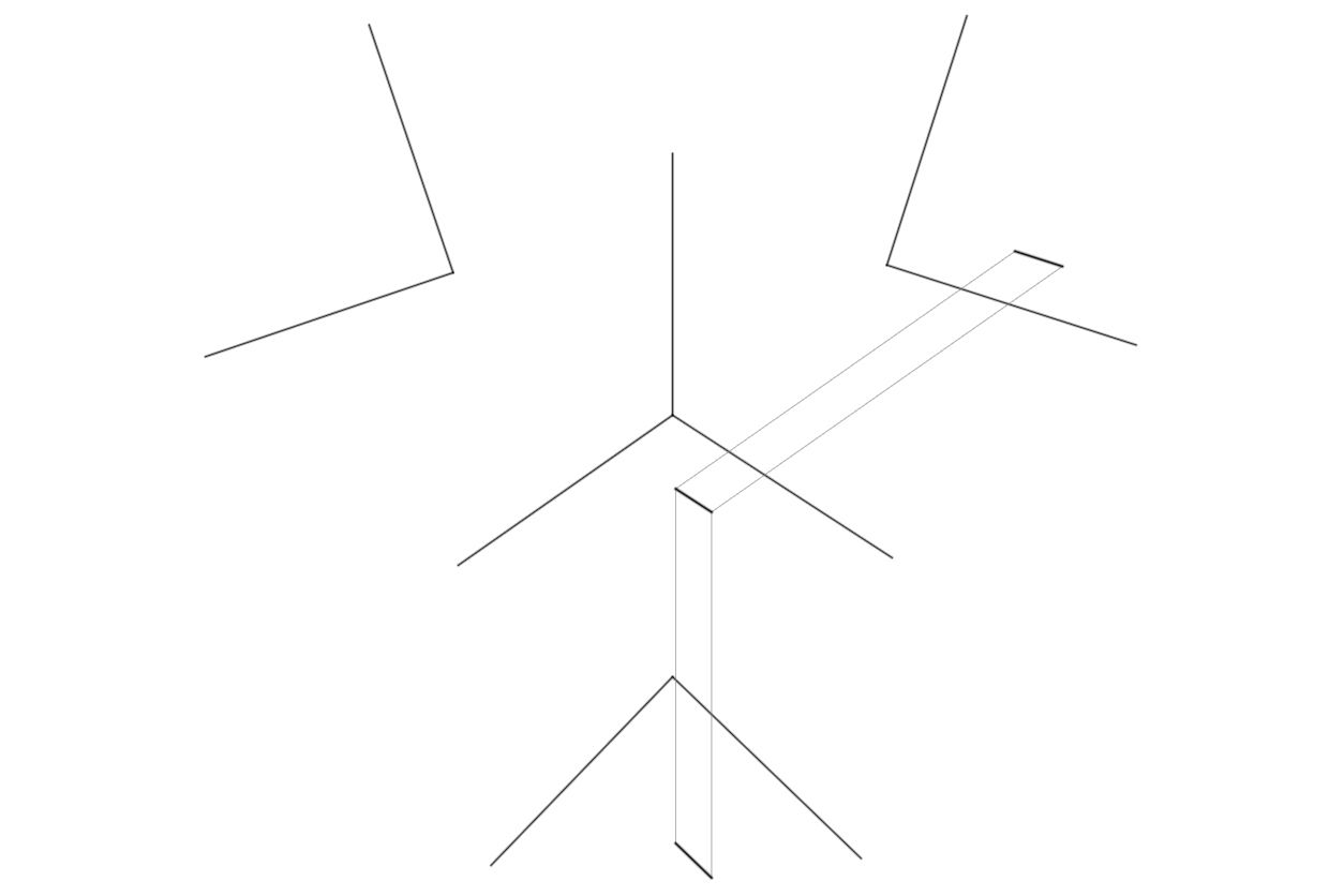
By Coordinate#
When drawing a line (or point) with its draw_line() method, the new line is returned from the function and can be assigned to a variable. Otherwise, existing lines are stored in the ReferencePlane.objects dictionary — in a list item with the key "lines".
>>> new_line = my_axo.xy.draw_line(Line.random_line("xy"))
>>> new_line.project(distance=20, ref_plane_key = "zx")
Line(Point(x=25.00, y=37.00, z=20.00), Point(x=68.00, y=37.00, z=20.00)) # notice z = 20.00
The projection of a line from a reference plane into the axonometric picture plane corresponds to defining the lines missing third coordinate: distance = 20.00 in the above listing. And as in the projection by reference plane the project() method has a parameter ref_plane_key = "zx" to select the auxilary reference plane to complete the projection. This parameter is not mandatory.
Note
This method comes very close to a projection by decomposition as described above.
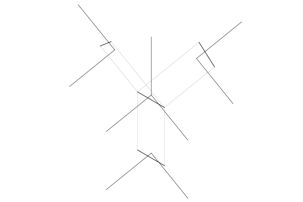
By Combination#
When a line is drawn between two points which share projections on others planes, the line is drawn there as well.
>>> line_1 = my_axo.draw_line(Line.random_line())
>>> line_2 = my_axo.draw_line(Line(Point.random_point(), Point.random_point()))
>>> my_axo.draw_line(Line(line_1.start, line_2.start))
>>> my_axo.draw_line(Line(line_1.end, line_2.end))
By Transformations#
Taking projection is a way to transpose objects from one dimension to another the images in the reference planes could be interpreted as the representations of higher dimensional objects.
The following methods allow you to implement this transformation in reverse, where points become lines and lines become surfaces: Point.project_into_line(), Line.project_into_surface().
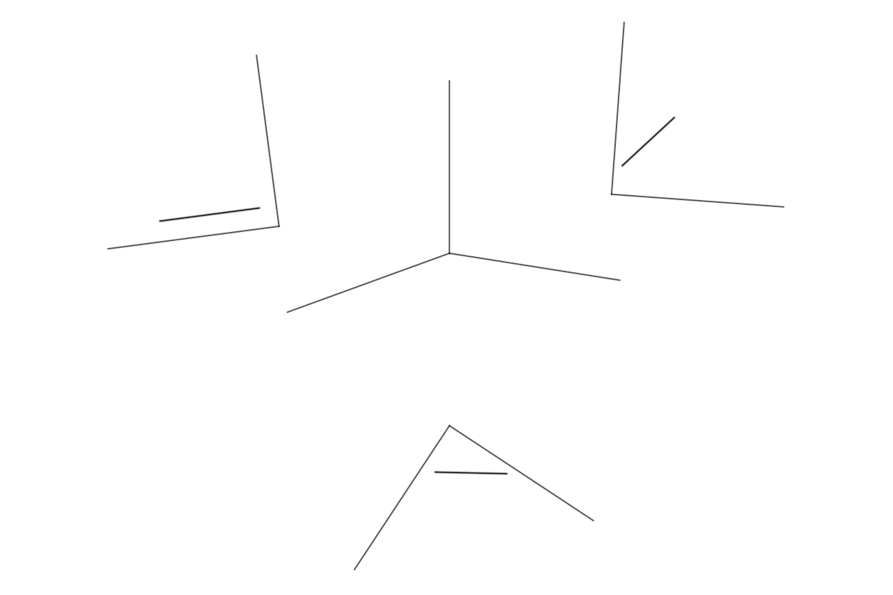
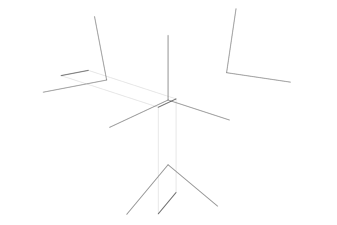
Points Become Lines#
>>> p_xy = my_axo.xy.draw_point(Point.random_point("xy"))
>>> p_xy.project_into_line(distance=50/2, length=50)
>>> p_yz = my_axo.yz.draw_point(Point.random_point("yz"))
>>> p_yz.project_into_line(distance=50/2, length=50)
>>> p_zx = my_axo.zx.draw_point(Point.random_point("zx"))
>>> p_zx.project_into_line(distance=50/2, length=50)
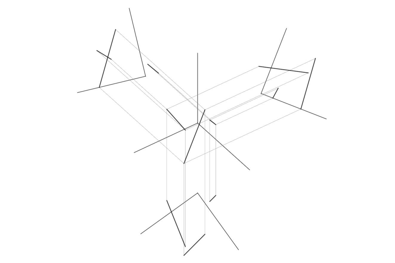
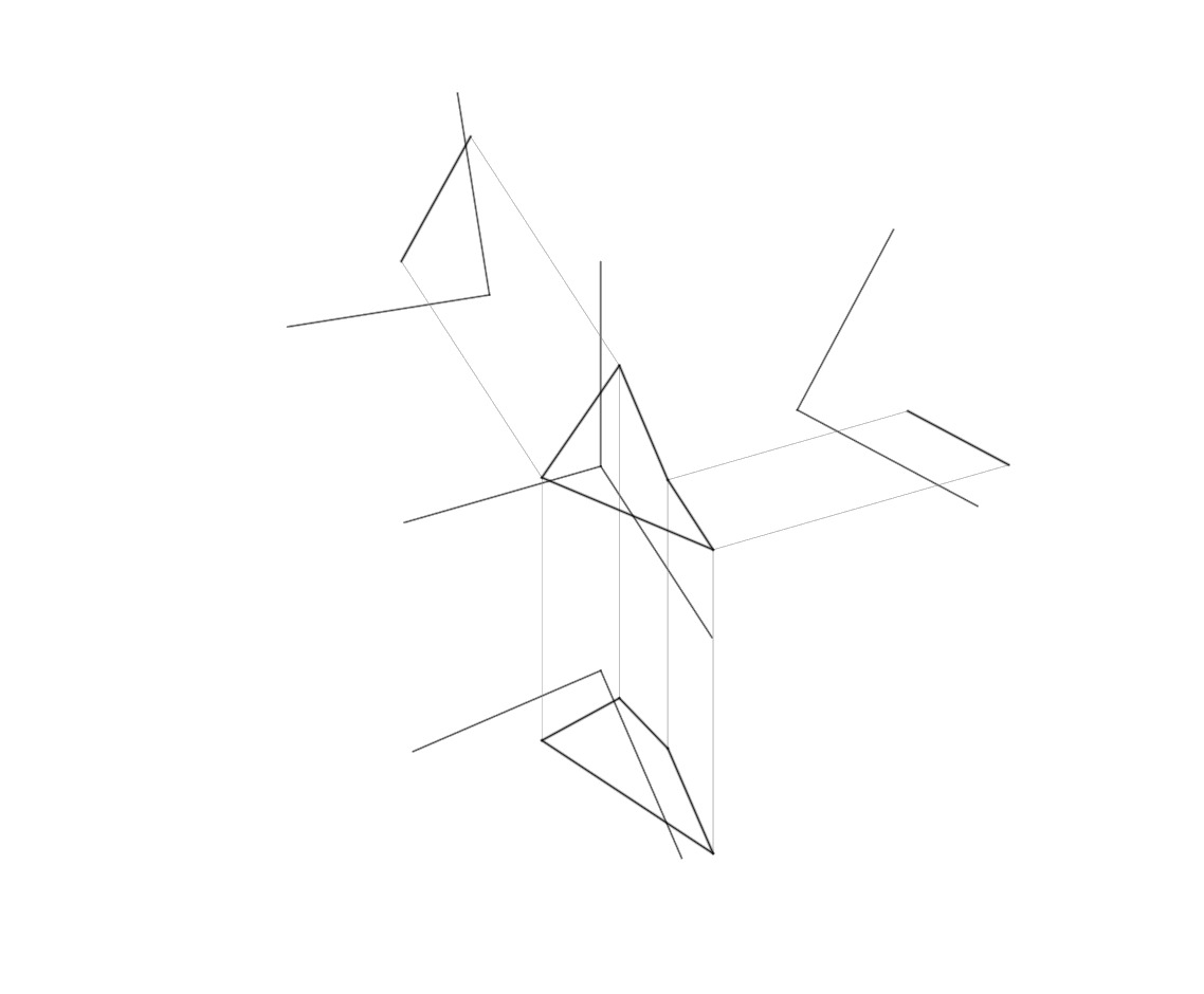
Lines Become Surfaces#
>>> l_xy = my_axo.xy.draw_line(Line(Point.random_point("xy"), Point.random_point("xy")))
>>> l_xy.project_into_surface(distance=50/2, length=50)
>>> l_yz = my_axo.yz.draw_line(Line(Point.random_point("yz"), Point.random_point("yz")))
>>> l_yz.project_into_surface(distance=50/2, length=50)
>>> l_zx = my_axo.zx.draw_line(Line(Point.random_point("zx"), Point.random_point("zx")))
>>> l_zx.project_into_surface(distance=50/2, length=50)
Preview Plotter Paths#
Since the primary intent of the axonometry library is to be oriented towards plotting, this command is straightforward.
>>> my_axo.show_paths()
c.f. Implementation
This command calls the vpype_viewer to render the internal Drawing object. The pen width is predefined in relation to the type of line (projection trace, geometry or coordinate systems). When plotting, however, the lines are treated as paths only and all other properties (such as width or style) are discarded.
Export Drawing#
When running axonometry, a new output folder is automatically created. The folder will be called output and will be located in the place where axonometry was installed (see install section). A custom path can be specified as a parameter in the various export functions.
Save SVG Files#
>>> my_axo.save_svg("filename", directory = "./output/")
Save PNG Files#
>>> my_axo.save_png("filename", directory = "./output/")
Import External Files#
Caution
This features are still under development.
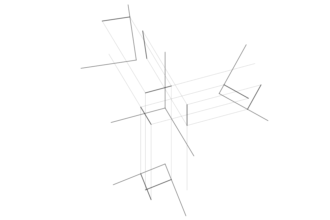
Import SVG Files On Reference Planes#
There are two steps to import an SVG file:
Selecting the reference plane with the help of the
Axonometry.xy,Axonometry.yzandAxonometry.zxattributes.Calling the
ReferencePlane.import_svg_file()method with the path to the file as an argument.
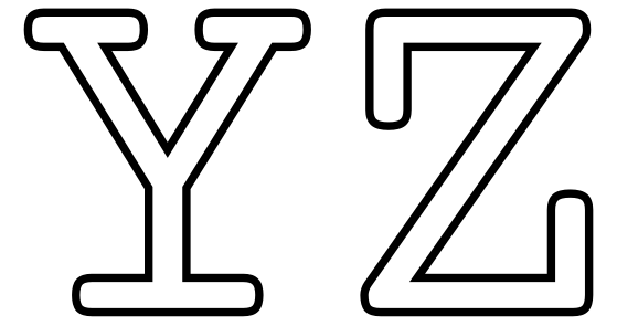
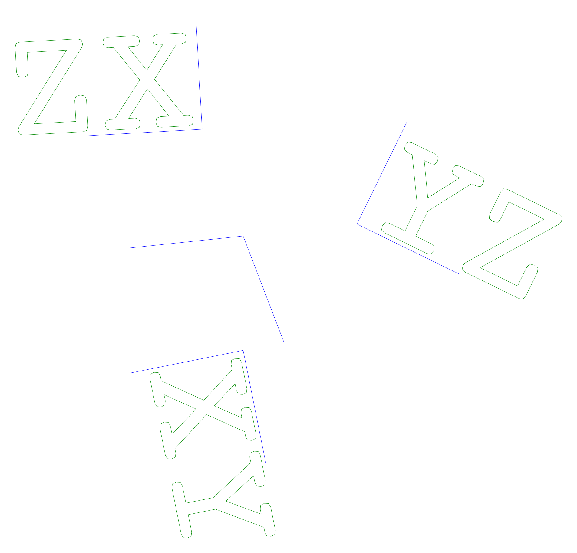
Input files must contain one or more SVG paths (Inkscape’s ‘Object to Path’ command comes in handy here). To demonstrate how the files are oriented in the reference planes, we will use the three corresponding reference plane coordinate letters. The following snippet loads one SVG file into each reference planes.
>>> my_axo.xy.import_svg_file("examples/xy.svg", scale=.3)
>>> my_axo.yz.import_svg_file("examples/yz.svg", scale=.3)
>>> my_axo.zx.import_svg_file("examples/zx.svg", scale=.3)


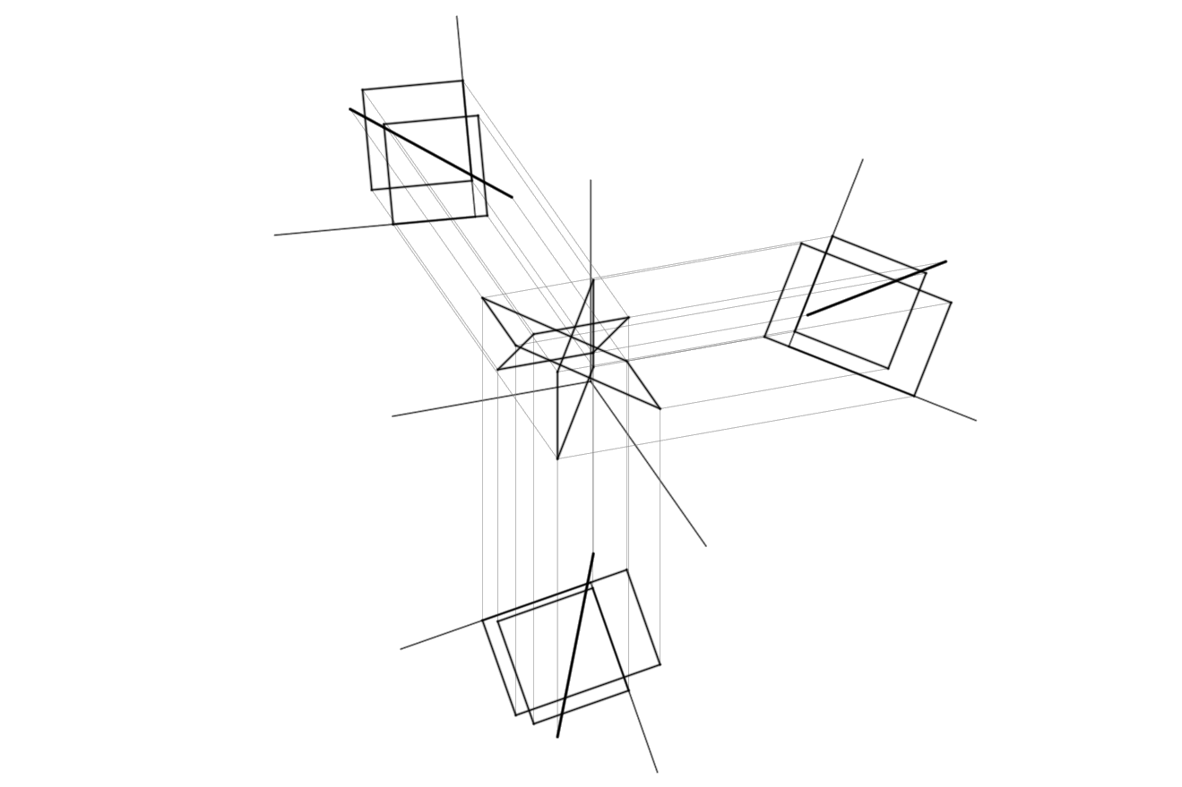
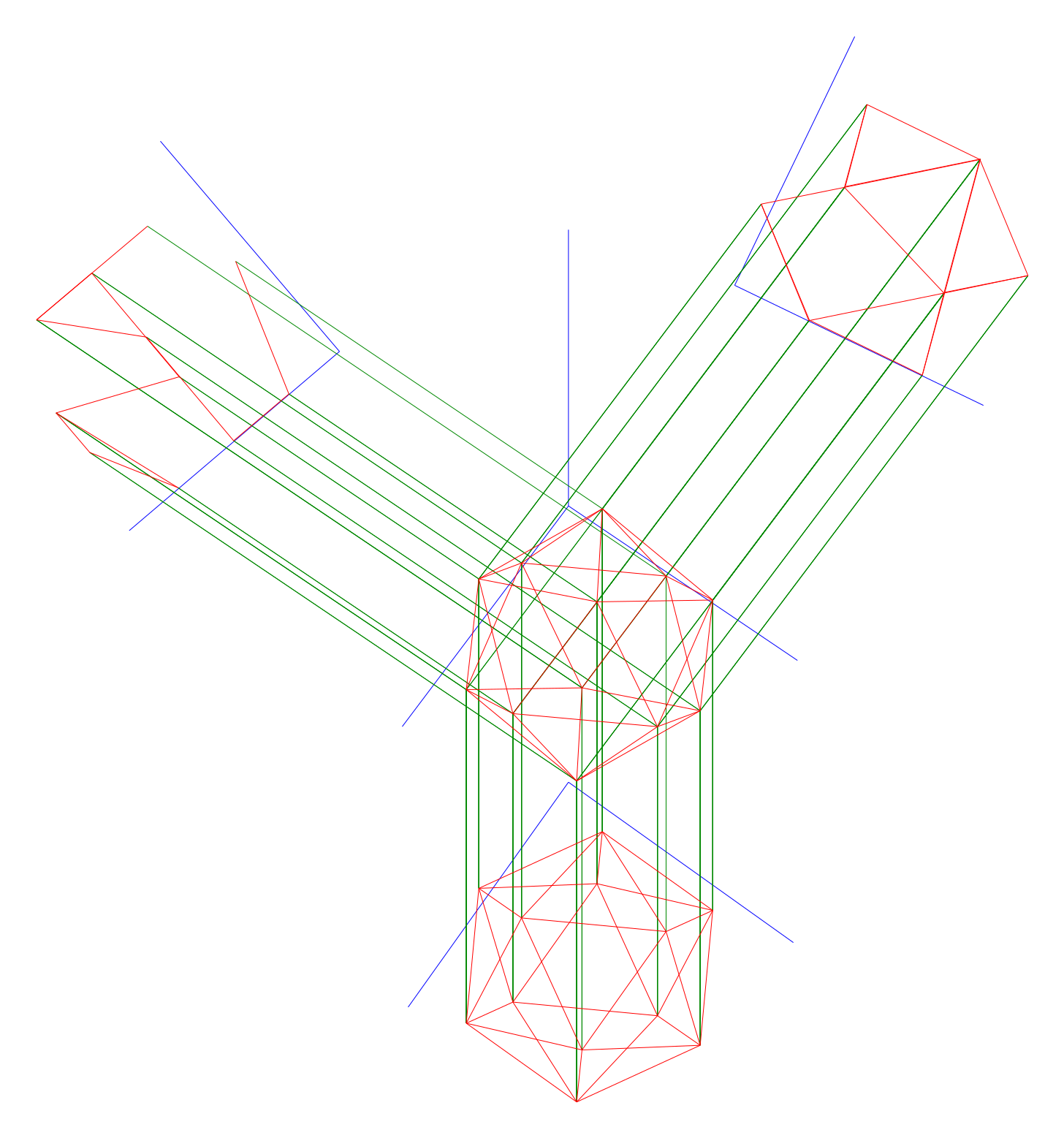
Import OBJ Files On Axonometric Picture Plane#
The OBJ file is the description of a 3D model. As it has three-dimensional coordinates, it is added directly to the axonometric image plane.
>>> my_axo.import_obj_file("./examples/icosphere.obj")
Hint
To export a model as an OBJ file from Blender, you need to tweak two things:
The position of the object’s origin. Most likely it is set by default to the objects center. Instead, try to set it to the world origin
(0,0,0).The forward and up axis settings in the export menu: try with
YandZ.