Walkthrough#
The axonometry library is designed for scripting. A script is a file written in Python with sequences of operations such as script.py. Running the script produces a vector drawing that can be displayed as an SVG file. The script is executed by passing the file to the python command in a terminal/shell. As stated in the installation section, the script can be executed with uv run --with axonometry script.py.
The following is a line by line explanation of such a script. The full script is at the bottom of this page. Copy its contents into a file (e.g. script.py) in order to run it. The images here are for illustration. Normally the axonometry.show_paths() function is only called at the end of the script.
Detailed documentation of the code blocks used are linked in the API Reference section.
1. Setup#
Import the axonometry library and initiate an Axonometry object.
Initiating the axonometry will automatically set up two elements:
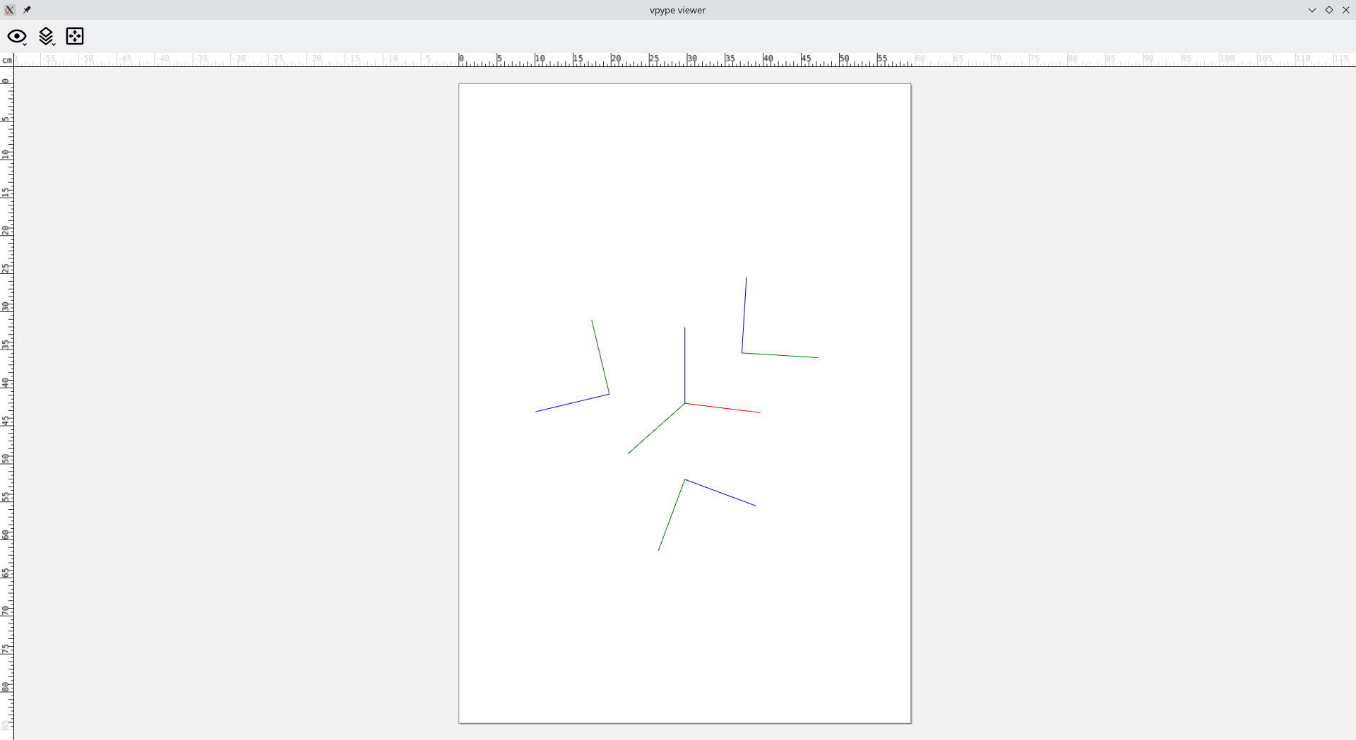
A reference trihedron represented by the traces of the three orthonometric coordinate planes in space. The three lines are the orthogonal projections of the X, Y and Z axes in space. Think of it like the corner of a cube. By default the trihedron is placed at the centre of the sheet. These lines are not used for drawing but are a spatial reference.
Three reference planes corresponding to each coordinate plane tilted into the axonometric picture plane. They represent the YX, YZ and ZX axes respectively.
The resulting axonometry is a combination of four planes. One axonometric picture plane and three reference planes. XYZ and (counterclockwise) XY, YZ, ZX respectively. These four planes are the basis for the drawing operations as they determine the location of the vraious objects, by specifying “where” to draw (i.e. adding geometric elements).
Attention
The vpype viewer could behave differently on certain systems. By opening the viewer, the execution of the script is halted. It can occur that after closing the vpype viewer window the script does not terminate properly. In that case, just hit CTRL+C to interupt the script.
2. Drawing#
The library is intended for plotting. In that sense, the base object to work with is the Line. There are two ways to create make lines. By adding them directly to planes or by projecting existing lines from one plane on another.
2.1 Adding geometry to planes#
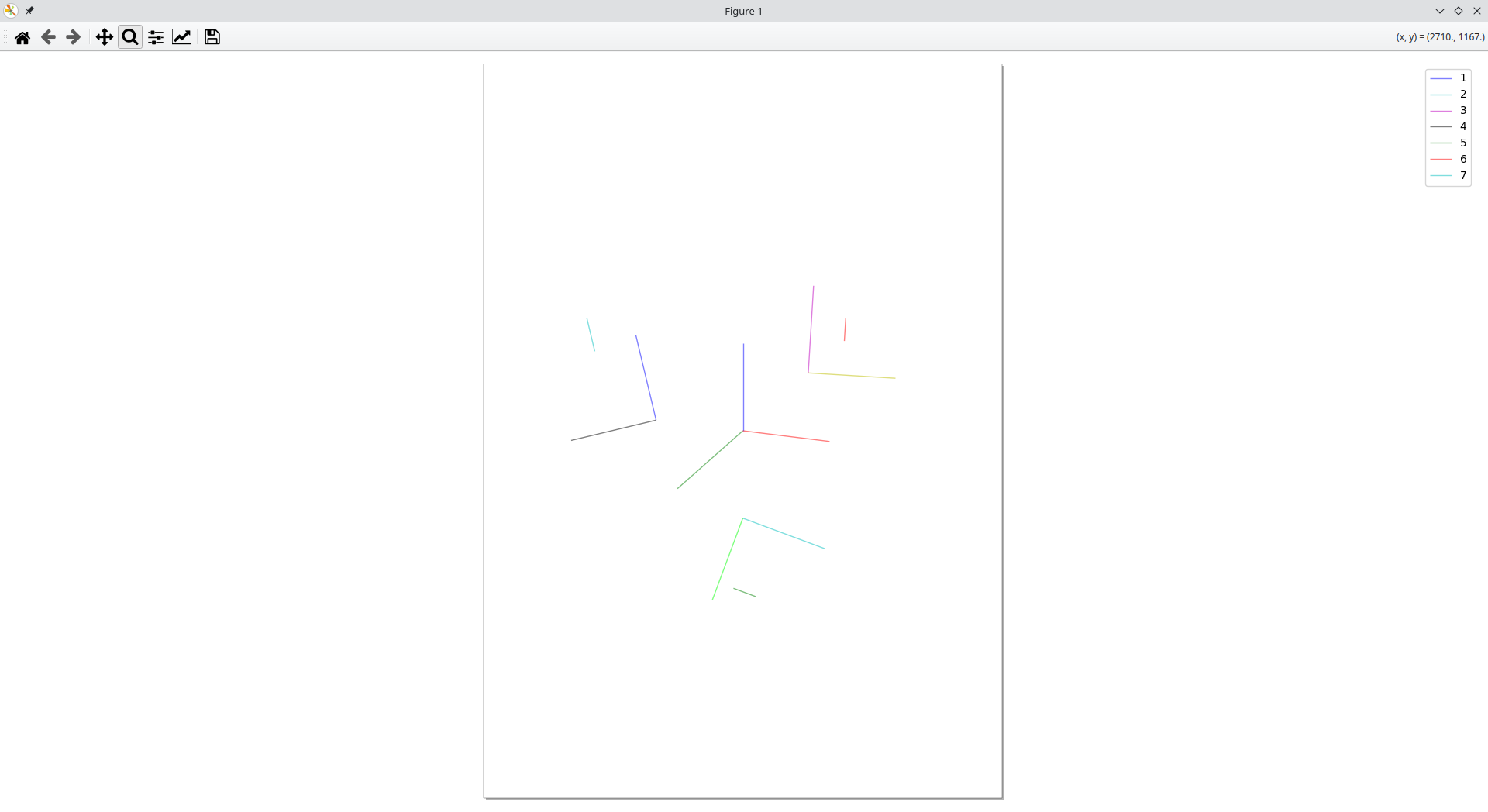
Lines are defined by their starting and ending Point. They can be added in a similar fashion to reference planes or the axonometry plane.
In order to draw with lines, one adds them to their respective plane. There three reference planes are accessed from the
Axonometryobject,my_axo, and a key of to their coordinates:xy,yzandzx.
Important
When adding geometry to planes, these objects (i.e. the Line and Point) have to be initiated with the corresponding parameters. In this case, the points of line_xy are defined by x and y coordinates: Line(axo.Point(x=98, y=93), axo.Point(x=55, y=46)) in order to be added to the XY reference plane: my_axo["xy"].draw_line(line_xy).
There’s one plane left to add lines to: the axonometry plane. In that case, the line object has to be defined by all three X, Y and Z coordinates.
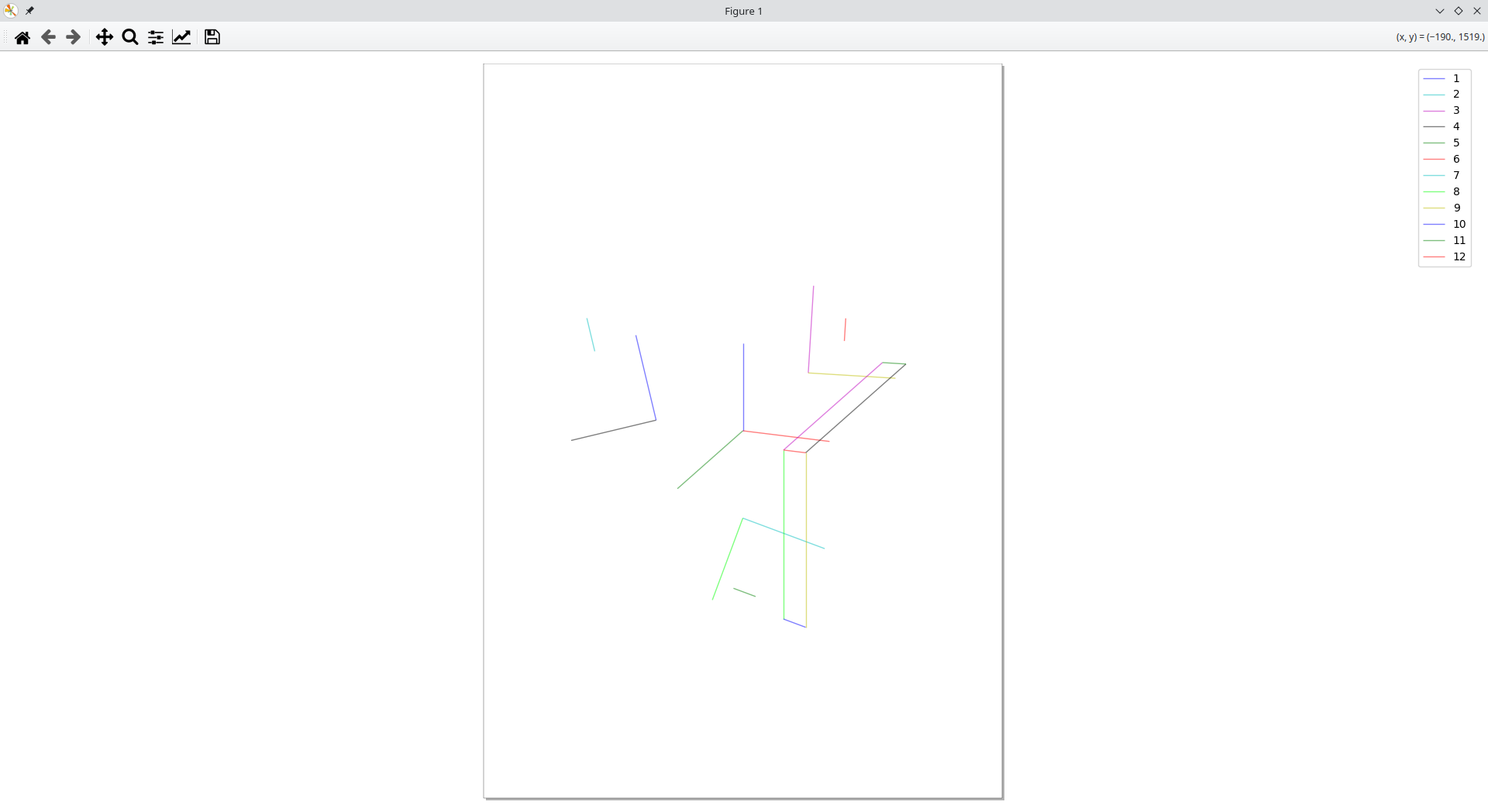
This is a special case as the Line object is being split in into two projections in order to be defined by intersection on the axonometric plane. This brings us to the next topic.
Note
The draw_line() function returns the added object.
2.2 Projecting geometry between planes#
In order to project a line, one hase to call the project() function and provide some additional parameters.
To project from a reference plane to the axonometry plane, one choses an object included in one of the reference planes, like
line_xyorline_zx, and calls the projection function with a distance value. This value is the third coordinate not defined in the current reference plane.
Note
By projecting a line from a reference plane into the axonometric plane, an auxiliary line is drawn in another reference plane to define the third coordinate. This is similar to adding a line directly in the axonometric plane.
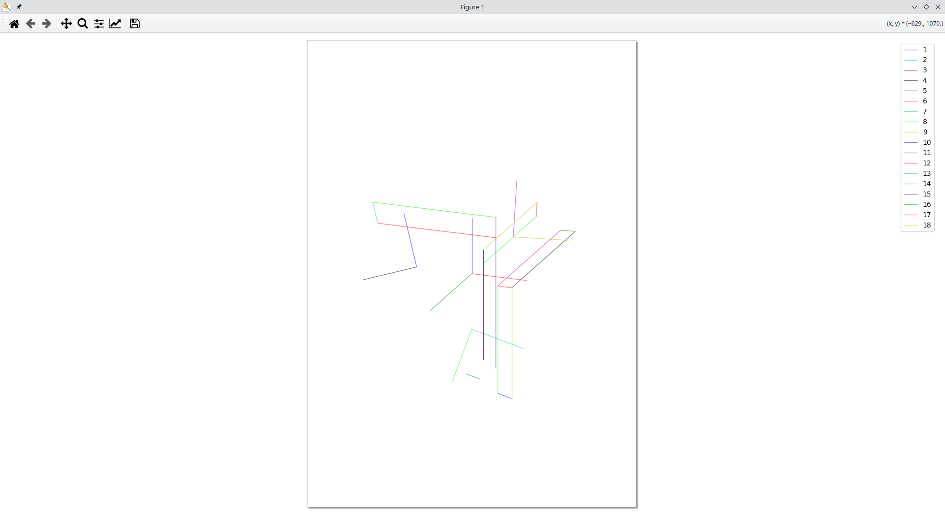
One can as well project the line from the axonometry plane onto one of the reference planes.
3. Collections#
There are as well various collections in order to access the different geometries:
The axonometry and reference planes have an
objectsattribute which is a list of the geometries in the respective plane.
{'points': [Point(x=92, y=84, z=17), Point(x=92, y=111, z=17), Point(x=92, y=84, z=17), Point(x=92, y=111, z=17), Point(x=79, y=45, z=82), Point(x=79, y=18, z=82), Point(x=79, y=45, z=82), Point(x=79, y=18, z=82), Point(x=44, y=39, z=39), Point(x=44, y=39, z=65), Point(x=44, y=39, z=39), Point(x=44, y=39, z=65), Point(x=50, y=65, z=93), Point(x=50, y=65, z=132), Point(x=50, y=65, z=93), Point(x=50, y=65, z=132)], 'lines': [Line(Point(x=92, y=84, z=17), Point(x=92, y=111, z=17)), Line(Point(x=79, y=45, z=82), Point(x=79, y=18, z=82)), Line(Point(x=44, y=39, z=39), Point(x=44, y=39, z=65)), Line(Point(x=50, y=65, z=93), Point(x=50, y=65, z=132))]}
[Point(x=79, y=45), Point(x=79, y=18), Point(x=79, y=45), Point(x=79, y=18), Point(x=92, y=84), Point(x=92, y=111), Point(x=92, y=84), Point(x=92, y=111), Point(x=92, y=84), Point(x=92, y=111)]
[Line(Point(y=39, z=39), Point(y=39, z=65)), Line(Point(y=84, z=17), Point(y=111, z=17)), Line(Point(y=45, z=82), Point(y=18, z=82)), Line(Point(y=65, z=93), Point(y=65, z=132))]
{'points': [Point(x=50, z=93), Point(x=50, z=132), Point(x=50, z=93), Point(x=50, z=132), Point(x=44, z=39), Point(x=44, z=65), Point(x=44, z=39), Point(x=44, z=65), Point(x=92, z=17), Point(x=92, z=17), Point(x=92, z=17), Point(x=92, z=17)], 'lines': [Line(Point(x=50, z=93), Point(x=50, z=132)), Line(Point(x=44, z=39), Point(x=44, z=65)), Line(Point(x=92, z=17), Point(x=92, z=17))]}
The geometries have an attribute
projectionswhich is a dictionary containing their projected pairs.
{'xy': Line(Point(x=92, y=84), Point(x=92, y=111)), 'yz': Line(Point(y=84, z=17), Point(y=111, z=17)), 'zx': Line(Point(x=92, z=17), Point(x=92, z=17)), 'xyz': []}
[Line(Point(x=44, y=39, z=39), Point(x=44, y=39, z=65))]
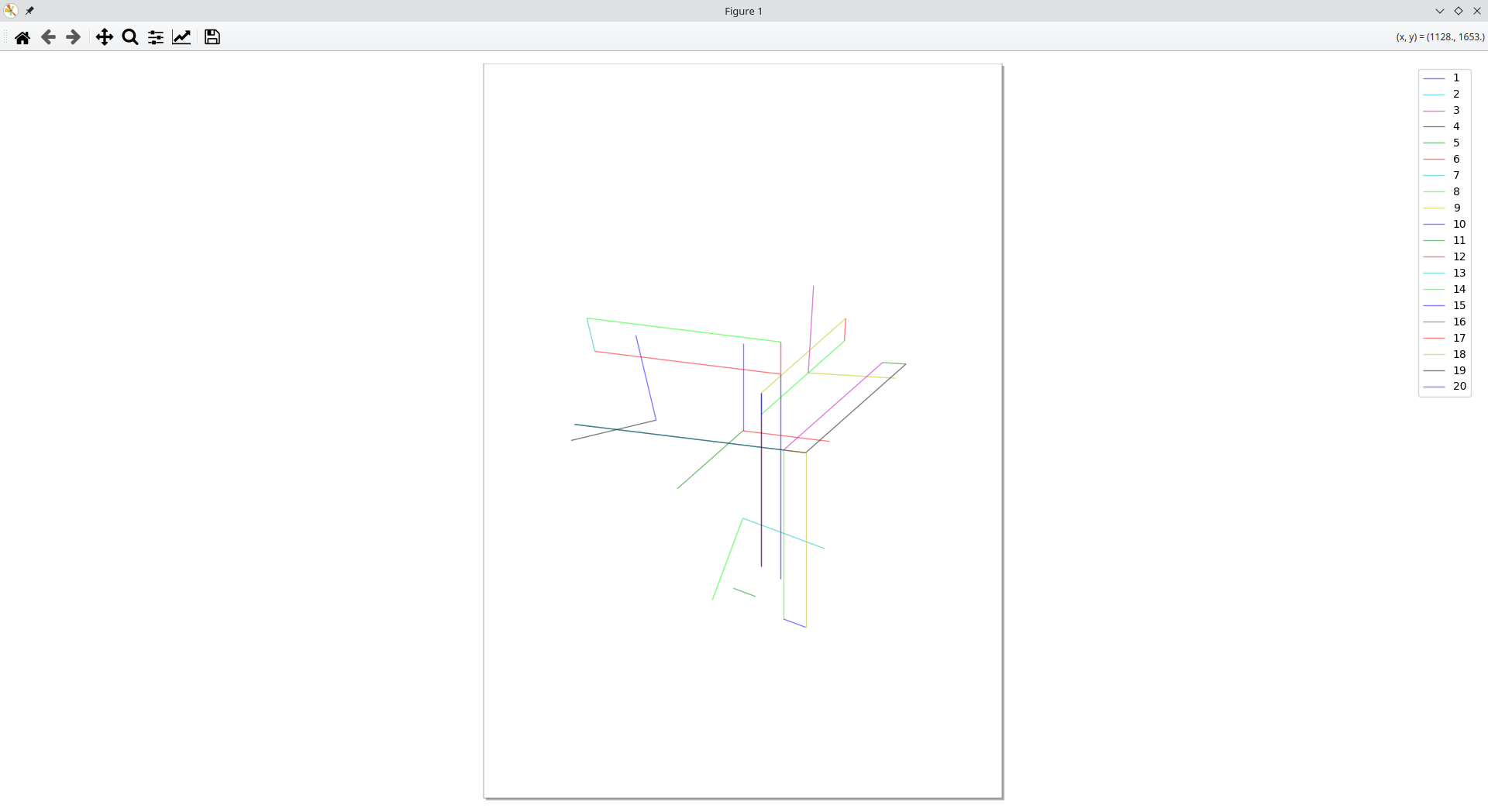
4. Display & Save#
Commonly at the end of the script, the generated drawing can be displayed and saved as an SVG file.
Note
The library is intended to generate axonometries to be sent to a pen plotter. In this sense, show_paths() is not intended to provide more information than where the plotter will draw a line. Line weights and the like are defined by the choice of drawing tool.
5. Full Script#
6. Running the Script#
From within the installation directory, run the script by invoking uv:
uv run script.py